
Setting of system parameters
To ensure a correct image processing by the system you should perform the following steps. Calibration (3.1.), setting of grey / color thresholds (3.2.) and setting of form parameter (3.3.) have to be done due to the different microscopy conditions separately in both modes: motility and morphology. You change the mode using the functions Database / Spermiogram Data and Database / Morphology Data.
Calibration
1. For calibration either an 100x100 µm grid (e.g Makler chamber ) or an object micrometer has to be put under the microscope.
2. Take a snapshot from the scale. Menu: Video / Snapshot.
3. Choose from the menu Options - Calibration
4. Draw a line between two positions on the scale. Click with the mouse onto the first position and then (with the left mouse button being pressed) draw a line to the second position. After this operation the calibration dialog opens.
5. Use the calibration dialog to transform the distance in pixel to a metric unit. Choose the relevant metric unit (µm, mm, cm). For calculations of concentrations (cells/ml) you have to set also the chamber depth.
6. For performance of a test measurement choose menu option Image / Count, You should see the measurement result in form of a table where the area value is assigned to a metric unit. Check the values for plausibility.
Setting of the grey level / colour intensity thresholds for image segmentation
The procedure is as follows: First take a still image by choosing Video / Snapshot. By choosing Option / Thresholds you can check the current thresholds and - if needed - set them by the slides. When having grey level images, the channels red and blue should be set to 0 (lower level) and 255 (upper level). The settings for grey level images are done by the green channel only. Using the preview function, the resulting image can be viewed on the screen. Set the thresholds in such a way that the objects appear (with highest contrast possible) dark on a bright background. Pushing the button Pseudo Live in preview mode shows the binary image in live mode.
To learn the object grey/colour level you can also use the automatic learning functions by pushing the Button Learn Object and Learn Back. In “Learn Object Mode” you can click in the object area and move the mouse over the object by holding down the left mouse button. By this all the object grey/colour values are added to the threshold range. The opposite operation can be done in the “Learn Back Mode”. In this mode all of the background grey/colour values are removed from the actual range.
Three learn modes are available lower fixed, upper fixed and band. In the band mode both lower and upper levels are adjusted.
Having dark objects on a bright background please select lower fixed. When you have bright objects on a dark background please select upper fixed. The band mode is useful when you have objects in an background with dark and although bright regions.
For increasing the object area you although have the button ¬® and for decreasing the object area you can choose the button ®¬.
You can inverse the threshold operation by checking the property “Invert”.
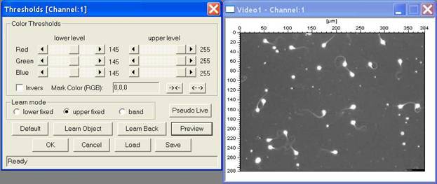
Fig. 3.1. Left: Dialog for setting the grey and colour thresholds. The video window on the right shows sperms in the current grey image.
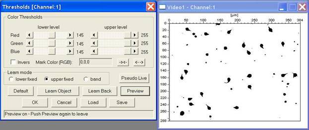
Fig. 3.2. Preview of the image after correct setting of thresholds for optimal check of sperm head for motility measurements.
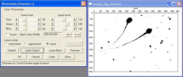
Fig. 3.3. Preview of the image after correct setting of thresholds for optimal check of sperm for morphology measurements.
Setting of form parameters for object recognition:
Form parameters are calculated continuously during image processing. By setting the proper upper and lower levels for these parameters unwanted objects can be excluded from being counted. For setting choose in the menu Options / Form parameter.
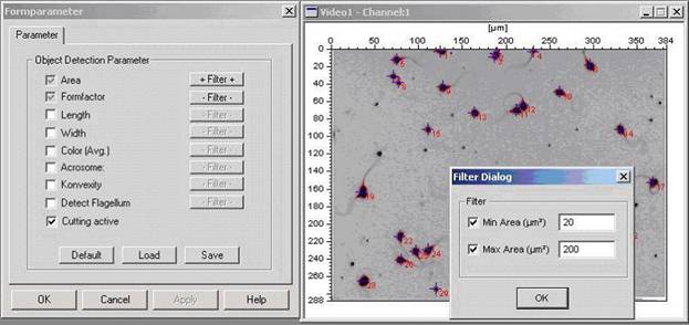
Fig. 3.4. Dialog for setting the form parameters for a motility and concentration measurement
Description of the from measuring parameters:
|
Area |
Object area calculated on the base of the contour. Due to the actual calibration the value is converted into metrical units. |
|
Formfactor: |
Value without unity which is calculated from the ratio of circumference and area. |
|
Length / Width: |
Maximum length and with calculated on the base of the contour. The value is converted into metrical units (same as area). |
|
Color (AVG): |
Mean color value of all the object pixels |
|
Acrosome: |
Measured parameter for the regularity of the color distribution (Homogenity) within the object |
|
Convexity: |
Value without unity calculated as a ratio of the length of the minimal convex cover and the length of the contour |
|
Flagellum: |
On the basis of available contour information the system decides whether the object has an appendix (flagellum ) or not. The limiting value for the decision (Max Value) should be between 0.4 -- 0.6. |
Cutting active: Activation of an algorithm to cut conglomerates. When two or more objects are within a cluster and are counted as one object this algorithm can divide the cluster and this leads to more realistic counting results:
 Fig. 3.5. Cutting
of 2 clustered sperms.
Fig. 3.5. Cutting
of 2 clustered sperms.
With the exception of the form parameters Area and Formfactor all form parameters can be activated or deactivated. The parameters Area and Formfactor are evaluated constitutively. By use of the button Filter the upper and lower level of the respective form parameter filter can be set.
Example: In Fig. 3.4. the filter for the form parameter area has been set for a minimum area of 20 µm² and for a maximum area of 200 µm². The unit µm has been selected during system calibration. With this setting, only objects will be counted which are >= 20 µm² and <= 200 µm².
Note:
The parameter settings are separately store for motility and morphology measurements. Please change to the desired mode an make the settings.
Standard settings of formparameter for motility (concentration) estimation:
Area and Formfactor on, All other formparameters off
Min Area: 10 µm² - Filter on
Max Area 40 µm² - Filter on
Standard settings of formparameter for morphology estimation:
Area on; Formfaktor on; Length on, Width on; Color (AVG) on and Acrosome on; All other formparameters off
Checking microscopy light conditions and automatic setting of the grey level / colour intensity thresholds for image segmentation
Proper setting of the grey/colour level thresholds is of utmost importance for automatic object recognition. Therefore, these settings should not be changed after having been set for a certain preparation. When the intensity of the microscopy light was changed the segmentation threshold settings have to be readjusted. So in medeaLAB an function for checking the microscope illumination brightness and comparing with the brightness of a reference image allows you to find the old settings. Menu: Options / Check Illumination:
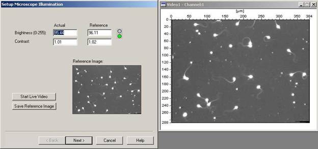
Fig. 3.1. First page of the dialog for checking the microscope illumination settings. The video window on the right shows sperms in the current grey image.
Push the Button “Start Live Video” and adjust the microscope brightness until the difference between the actual image and the reference image is smaller than 5%. In this case the green light goes on.
To store a new reference image please push the button “Save Reference Image”.
Push the button “Next” when ready.
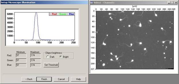
Fig. 3.2. Second page of the of the dialog for checking the microscope illumination settings dialog
On this side of the dialog you can automatically set the grey/colour level thresholds for object detection. A grey/colour histogram in which the ranges of the grey value distribution is shown. Select first if the objects are more brighter or darker than the background: Radio Button Object brightness Dark or Bright. Than you can set the system threshold by pushing the button “Set Threshold”. Finish the dialog by pushing the button “Finish”
Counting of objects for evaluation the form parameters:
In order to prove the correct setting of thresholds and form parameters: Start a measurement (after activation of the image window) by choosing from the menu: Image / Count.
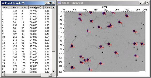
Fig. 3.5. Count evaluation
Your filter settings are correct if all sperms displayed in the video window are marked and listed in the table.
All changes of your optical system which affect the illumination of your field of view are critical for these filter settings. You therefore should always check your filter settings after having changed your system.
Setting and control of the system options for tracking
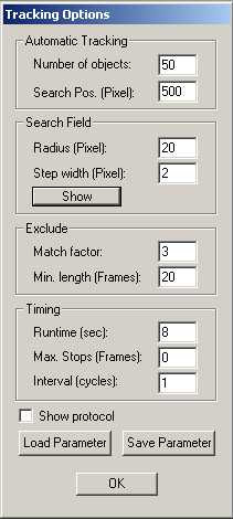
Activate the tracking window and choose the option Options / Tracking Options from the menu. The duration (in seconds) of the tracking measurement can be set by Timing - Runtime (sec). For the measurement of sperm motility the settings shown below have proven as a good default:
|
Fig. 3.7. Dialog for setting the system parameters needed for motility analysis
|
Number of objects: to be tracked simultaneously. This value depends on the performance of your computer and should be set between 50 and 100.
Search Pos.: Number of search positions in the image where the system searches for objects using random generated positions. Radius: of the search area used to find the new object position during tracking. Step width: of search positions within the search area (should be smaller than object sizes). Button Show: makes the search field visible in the video image Match factor: A factor calculated during tracking to check the object parameters, e.g. to identify collisions of objects. A large match factor makes the system less sensible. Min. length: Motile objects which have been tracked for a short time (in frames) will be excluded from evaluation. Runtime: Time during which the system is running. Max. Stops: The number of frames, during which an object does not move, before it is excluded from further evaluation. Interval cycles: Allows reduction of temporal resolution. For CASA applications it has to be set to 1 for maximal resolution. Show protocol: not available for CASA use |
Setting and control of the thresholds for classification according to the WHO-categories[1]
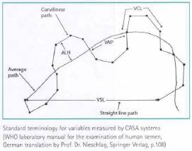
VCL = curvilinear velocity (µm/s). Time–average velocity of a sperm head along its actual curvilinear path, as perceived in two dimensions in the microscope.
VSL = straight-line velocity (µm/s). Time–average velocity of a sperm head along the straight line between its first detected position and its last.
VAP = average path velocity (µm/s). Time–average velocity of a sperm head along its average path. This path is computed by smoothing the actual path according to algorithms in the CASA instrument: these algorithms vary between instruments.
ALH = amplitude of lateral head displacement (µm/s). Magnitude of lateral displacement of a sperm head about its average path. It can be expressed as a maximum or an average of such displacements. Different CASA instruments compute ALH using different algorithms, so that values are not strictly comparable.
LIN = linearity. The linearity of a curvilinear path. VSL/VCL.
WOB = wobble. Measure of oscillation of the actual path about the average path, VAP/VCL.
In order to relate the monitored sperm trajectories to the various WHO-categories, some thresholds have to be set properly. Choose Spermiogram / Thresholds
or
Toolbar: ![]()
The presentation of sperm tracks is described in the following:
|
Classification |
WHO-category |
Color |
Color (RGB) |
|
Fast linear progressive motile |
(„a“) |
green |
0,255,0 |
|
Slow linear progressive motile |
(„b“) |
yellow |
255,255,0 |
|
Local motile |
(„c“) |
red |
255,0,0 |
|
Circle swimmer |
(„c“) |
blue |
0,0,255 |
|
Not motile |
(„d“) |
black |
0,0,0 |
|
|
VAP* (Motile/not motile): The minimum velocity, which qualifies an object as motile. (Also not motile objects conditionally show minimal position changes by camera noise)
VAP* (Progessive): velocity which qualifies a motile object as progressive. WHO ³ 5 µm/s
VAP* (Fast/Slow):velocity which qualifies a motile object as fast. WHO ³ 25 µm/s at 37°C or ³ 20 µm/s at 20°C.
Linearity: Ratio of the shortest distance between start and endpoint of the recorded sperm movement to the trajectory length of the track.
Radius circle swimmers: Minimum and maximum radius of circle swimmers.
* VAP = Velocity average path linear |
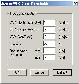
Fig. 3.6. Dialog for setting the parameters needed for track classification
The classification of the sperms into the WHO-Classes works in the following order:
1. A sperm, which swims with an Average Path Velocity (VAP) lower than the threshold for VAP (Motile/not motile) is classified as not motile (WHO-D).
2. If the VAP of the sperm is higher as the threshold for VAP (Motile/not motile) but smaller than the threshold for VAP (Progressive), then that sperm is classified as local motile (WHO-C).
3. As circle swimmer is also classified as WHO-C.
4. If the VAP of the sperm is lower than the threshold VAP (Fast/Slow) it is classified as slow motile (WHO-B).
5. If the movement of the sperm is not straight and the linearity is lower then the linearity threshold it is also classified as WHO-B.
6. All sperms swimming faster than the threshold for (Fast/Slow) are classified as fast linear progressive motile (WHO-A).